Lasso Regression
Detecting and handling multicollinearity using L1 regularization
What is Lasso Regression?
Least Absolute Shrinkage and Selection Operato Regression, also known as L1 Regularization or Lasso Regression, is a type of linear regression that uses a regularization term to prevent overfitting. In other words, it’s a regression algorithm that minimizes the influence unuseful features towards zero. Thus, it can be very effective at handling data that suffers from severe multicollinearity. When multicollinearity occurs within the dataset, least squares estimates can be unstable and have high variance.
Note that the important keywords: high variance, multicollinearity, overfitting, regularization, and unstable.
-
High variance is a situation where the model estimates can vary a lot even when the data is slightly changed.
-
Multi-collinearity is a situation where there are high correlations between two or more features.
-
Overfitting is a situation where the model learns the training data too well that it fails to generalize to the test data. So, when the model sees unseen data, it will perform poorly.
-
Regularization is a technique that prevents the model from learning the training data too well or catching all the noises in the data by adding a penalty term to the cost function.
-
Unstable is a situation where the model estimates can vary a lot even when the data is slightly changed.
Now we know what Lasso Regression is and what it does, let’s see how it works from the mathematical perspective.
Mathematics Behind Lasso Regression
In Lasso Regression, we are going to use the same linear function that Linear Regression uses:
Similar to what we did in the Linear Regression post and the Logistic Regression post, we need to estimate the best and using the Gradient Descent algorithm. What the Gradient Descent algorithm does is to update the and values based on the cost function and the learning rate.
This example is just a simple linear model, we are going to use the following equations to update intercept and coefficient:
where is the learning rate, is the -th parameter, is the cost function, and is the -th feature.
Since we only have and , we can simplify the equation above to:
However, the only difference in Lasso Regression is that we are going to add a penalty term to the cost function. This penalty term is the sum of the absolute values of the weights multiplicated by the regularization term or weight. This is also known as the L1 norm of the weights.
The cost function for Lasso Regression that we have to minimize is given by:
where
- is Mean Squared Error.
- is the regularization parameter.
- is the L1 norm of the weights.
What’s Wrong with the Data?
In this post, we are going to use the Californian Housing Dataset from the Scikit-Learn library. For more details, you can check the official documentation or the dataset repository on StatLib.
from sklearn.datasets import fetch_california_housing
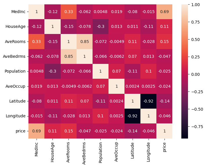
data = fetch_california_housing()df = pd.DataFrame(data.data, columns=data.feature_names)Let’s plot the heatmap to see the correlation between the features.

From the heatmap itself, we can notice that there are some features that are highly correlated with each other.
-
AveRoomsandAveBedrms: Higher average rooms may be associated with more average bedrooms. -
LatitudeandLongitude: The geographical location of the house.
However, there are more, we can’t just notice it in plain sight.
Let’s process df.corr() even more to see how features are correlated with each other.
df.corr()[df.corr() < 1].unstack().transpose().sort_values(ascending=False).drop_duplicates()| Variable 1 | Variable 2 | Correlation Coefficient |
|---|---|---|
| AveBedrms | AveRooms | 0.847621 |
| MedInc | AveRooms | 0.326895 |
| Latitude | AveRooms | 0.106389 |
| Population | Longitude | 0.099773 |
| Population | AveOccup | 0.069863 |
| … | … | … |
Here is a guide on how to interpret the values in the table above:
- Two or more features said to have a strong positive correlation if the correlation coefficient is close to .
- Two or more features said to have a moderate positive correlation if the correlation coefficient is close to .
- Two or more features said to have a weak positive correlation if the correlation coefficient is close to .
- Two or more features said to have a moderate negative correlation if the correlation coefficient is close to .
- Two or more features said to have a strong negative correlation if the correlation coefficient is close to .
You would notice that AveRooms and AveBedrms have a strong positive correlation.
Why would having two features with a high correlation coefficient be a problem?
Since these two features are highly correlated, meaning that if AveRooms increases, AveBedrms is also likely to increase.
Therefore, the model might be confused about which feature to use to predict the target variable.
There is also another approach Variance Inflation Factor (VIF) to determine what features suffer from multicollinearity. Let’s calculate VIF to see the correlation between the features. Determining VIF can be done with the following:
from statsmodels.stats.outliers_influence import variance_inflation_factor
vif_data = pd.DataFrame()vif_data["feature"] = data.feature_namesvif_data["VIF"] = [variance_inflation_factor(df.values, i) for i in range(len(data.feature_names))]print(vif_data)| feature | VIF |
|---|---|
| MedInc | 19.624998 |
| HouseAge | 7.592663 |
| AveRooms | 47.956351 |
| AveBedrms | 45.358192 |
| Population | 2.936078 |
| AveOccup | 1.099530 |
| Latitude | 568.497332 |
| Longitude | 640.064211 |
Here is a guide on how to interpret VIF values:
- : The feature is said to have no multicollinearity.
- : The feature is said to have a moderate multicollinearity.
- : The feature is said to have a severe multicollinearity.
From the heatmap, the correlation table, as well as the VIF table,
it’s clear that MedInc, AveRooms, AveBedrms, Latitude, and Longitude suffer from multicollinearity.
Let’s see how Lasso Regression can handle this problem.
Implementation
Let’s prepare the data for the Ridge Regression model by splitting the dataset into training and testing sets, and standardizing the feature values.
from sklearn.datasets import load_diabetes
data = load_diabetes()X, y = data.data, data.target
X_train, X_test, y_train, y_test = train_test_split(X, y, test_size=0.2, random_state=42)
scaler = StandardScaler()X_train_scaled = scaler.fit_transform(X_train)X_test_scaled = scaler.transform(X_test)Now out data is ready, we want pick a number of epoch, meaning how many times our model has to go through the dataset. In this example, we are going to use epochs, and it might take sometime. However, epochs should be enough to see the changes in the loss, intercept, and coefficients. Then we initialize the history of the loss, intercept, and coefficients so that we can visualize the changes in the values of these variables.
epochs = 100_000loss_history = list()intercept_history = list()coefficients_history = np.zeros((scaled_X.shape[1], epochs)) Next, we would need two helper functions: predict and loss_function.
Make sure to use vectorized operations to make the code faster.
Remember, regularization_term is the in the cost function.
def predict(intercept: float, coefficient: list, data: list) -> list: return intercept + np.dot(data, coefficient)
def loss_function(coefficients, errors, regularization_term): return np.mean(np.square(errors)) + regularization_term * np.sum(np.abs(coefficients)) We also need a function called soft_threshold to update the coefficients. There are three conditions:
- If the coefficient is less than the negative of the regularization term, then we subtract the regularization term from the coefficient.
- If the coefficient is greater than the regularization term, then we subtract the regularization term from the coefficient.
- If the coefficient is between the negative and positive regularization term, then we set the coefficient to zero.
def soft_threshold(coefficient, regularization_term): if coefficient < -regularization_term: return (coefficient + regularization_term) elif coefficient > lambda_: return (coefficient - regularization_term) else: return 0def lasso_regression( x, y, epochs, learning_rate = 0.1, regularization_term = 0.001): intercept, coefficients = 0, np.zeros(x.shape[1]) length = x.shape[0]
intercept_history.append(intercept) coefficients_history[:, 0] = coefficients loss_history.append(loss_function(coefficients, y, regularization_term))
for i in range(1, epochs): predictions = predict(intercept, coefficients, x) errors = predictions - y intercept = intercept - learning_rate * np.sum(errors) / length intercept_history.append(intercept)
for j in range(len(coefficients)): gradient = np.dot(x[:, j], errors) / length temp_coef = coefficients[j] - learning_rate * gradient coefficients[j] = soft_threshold(temp_coef, regularization_term) coefficients_history[j, i] = coefficients[j]
loss_history.append( loss_function( coefficients, errors, regularization_term ) )
return intercept, coefficients
intercept, coefficients = lasso_regression(scaled_X, data.target, epochs)Model Comparison
| Baseline | Ours | |
|---|---|---|
| MSE | 0.5482 | 0.5325 |
| MedInc | 0.8009 | 0.7769 |
| HouseAge | 0.1270 | 0.1248 |
| AveRooms | -0.1627 | -0.1288 |
| AveBedrms | 0.2062 | 0.1687 |
| Population | 0.0000 | 0.000 |
| AveOccup | -0.0316 | -0.0294 |
| Latitude | -0.7901 | -0.7960 |
| Longitude | -0.7556 | -0.7595 |
From the table, we can see the differences in the coefficients between the baseline model and the Lasso Regression model we developed are very minimal. Not bad, right?
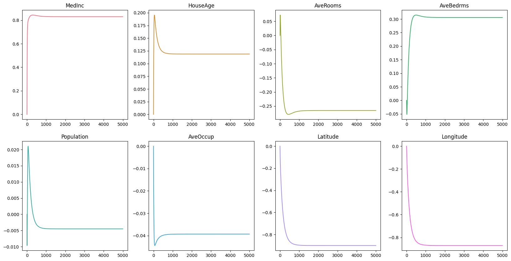
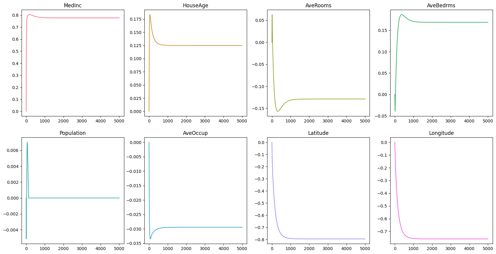
Now, let’s visualize the changes in the loss, intercept, and coefficients over time.


Remember that in the early section MedInc, AveRooms, AveBedrms, Latitude, and Longitude suffer from multicollinearity.
From the graph, we can see that the coefficients of MedInc seems to be the only feature left that has a significant impact on the target variable.
The coefficients of AveRooms, AveBedrms, Latitude, and Longitude are close to zero, and that indicates that these features are not important in predicting the price of the house.
Conclusion
Here are the key takeaways from this post:
- Lasso Regression is a type of linear regression that uses a regularization term to prevent multicollinearity.
- It uses the sum of the absolute values of the weights multiplicated by the regularization term to minimize coefficients.
- It will set coefficients to exactly zero.
- It can be used to select important features in the dataset.
- It can increase the model’s interpretability.
For the baseline model, you could see the code here. For own custom Lasso Regression model, you could see the code here.
Reference
- JMP. What is Multicollinearity? https://www.jmp.com/en_is/statistics-knowledge-portal/what-is-multiple-regression/multicollinearity.html
- Scikit-Learn. California Housing Dataset. https://scikit-learn.org/stable/datasets/real_world.html#california-housing-dataset
- StatsModel. Variance Inflation Factor. https://www.statsmodels.org/stable/generated/statsmodels.stats.outliers_influence.variance_inflation_factor.html
- NBSHARE. How to Use Pandas Correlation Matrix. https://www.nbshare.io/notebook/394171759/How-To-Use-Pandas-Correlation-Matrix/