Ridge Regression
Detecting and handling multicollinearity using L2 regularization
What is Ridge Regression?
Ridge Regression, also known as L2 Regularization or Tikhonov Regularization, is a type of linear regression that uses a regularization term to prevent overfitting just like Lasso Regression. The only difference is that Ridge Regression uses the sum of the squares of the weights instead of the sum of the absolute values of the weights.
Due to the square term, it minimizes the weights close to zero but not exactly zero. Thus, all the features will be used in the model. Moreover, Ridge Regression is good at when we have data in which the multicollinearity issue is not too severe.
Mathematics Behind Ridge Regression
In Ridge Regression, we are going to use the same linear function that Linear Regression uses:
Similar to what we did in previous posts, we need to estimate the best and using the Gradient Descent algorithm. What the Gradient Descent algorithm does is to update the and values based on the cost function and the learning rate.
This example is just a simple linear model, we are going to use the following equations to update intercept and coefficient:
where is the learning rate, is the -th parameter, is the cost function, and is the -th feature.
Since we only have and , we can simplify the equation above to:
However, the only difference in Ridge Regression is that we are going to add a penalty term to the cost function. This penalty term is the sum of the absolute values of the weights. This is also known as the L2 norm of the weights. The cost function for Ridge Regression that we have to minimize is given by:
where
- is Mean Squared Error.
- is the regularization parameter.
- is the L2 norm of the weights.
What’s Wrong with the Data?
Unlike the Lasso Regression post, we are going to use the Diabetes dataset from the Scikit-Learn library. For more details, you can check the official documentation.
from sklearn.datasets import load_diabetes
data = load_diabetes()feature_names = ['age', 'sex', 'body_mass_index', 'blood_pressure', 'serum_cholesterol', 'ldl', 'hdl', 'cholesterol_ratio', 'triglycerides', 'blood_sugar']There are ten features in the dataset. Let’s decipher what some features represent:
-
body_mass_index: It’s a measure of body fat based on height and weight. -
serum_cholesterol: The amount of cholesterol present in the blood. -
ldl: Low-density lipoprotein cholesterol, often referred to as “bad” cholesterol. -
hdl: High-density lipoprotein cholesterol, often referred to as “good” cholesterol. -
cholesterol_ratio: A ratio calculated by dividing the total cholesterol by the HDL cholesterol level. -
triglycerides: A type of fat found in the blood, expressed in logaritm. -
blood_sugar: The amount of glucose present in the blood.
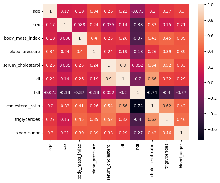
Let’s plot the heatmap to see the correlation between the features.

Here is a guide on how to interpret the values in the table above:
- Two or more features said to have a strong positive correlation if the correlation coefficient is close to .
- Two or more features said to have a moderate positive correlation if the correlation coefficient is close to .
- Two or more features said to have a weak positive correlation if the correlation coefficient is close to .
- Two or more features said to have a moderate negative correlation if the correlation coefficient is close to .
- Two or more features said to have a strong negative correlation if the correlation coefficient is close to .
Looking at the heatmap, we can determine easily what features are correlated with each other.
-
ldlandserum_cholesterolhave a strong positive correlation. -
ldlandcholesterol_ratiohave a strong positive correlation. -
serum_cholesterolandcholesterol_ratiohave a moderate positive correlation. -
serum_cholesterolandtriglycerideshave a moderate negative correlation.
These are the features that can be detected easily from the heatmap. With the following code, we can list out all the correlation values between the features.
df.corr()[df.corr() < 1] .unstack() .transpose() .sort_values(ascending=False) .drop_duplicates()| Variable 1 | Variable 2 | Correlation |
|---|---|---|
| ldl | serum_cholesterol | 0.896663 |
| cholesterol_ratio | 0.659817 | |
| cholesterol_ratio | triglycerides | 0.617859 |
| serum_cholesterol | cholesterol_ratio | 0.542207 |
| triglycerides | 0.515503 | |
| … | … | … |
| sex | hdl | -0.379090 |
| triglycerides | hdl | -0.398577 |
| hdl | cholesterol_ratio | -0.738493 |
We can also use Variance Inflation Factor (VIF) to determine the multicollinearity between the features.
from statsmodels.stats.outliers_influence import variance_inflation_factor
vif_data = pd.DataFrame()vif_data["feature"] = feature_namesvif_data["VIF"] = [variance_inflation_factor(df.values, i) for i in range(len(data.feature_names))]print(vif_data)| feature | VIF |
|---|---|
| age | 1.217307 |
| sex | 1.278071 |
| body_mass_index | 1.509437 |
| blood_pressure | 1.459428 |
| serum_cholesterol | 59.202510 |
| ldl | 39.193370 |
| hdl | 15.402156 |
| cholesterol_ratio | 8.890986 |
| triglycerides | 10.075967 |
| blood_sugar | 1.484623 |
Here is a guide on how to interpret VIF values:
- : The feature is said to have no multicollinearity.
- : The feature is said to have a moderate multicollinearity.
- : The feature is said to have a severe multicollinearity.
From the heatmap, the correlation table, as well as the VIF table, it’s clear that
ldl, serum_cholesterol, hdl, cholesterol_ratio, and triglycerides have a severe multicollinearity.
Let’s see how Ridge Regression can help us to solve this issue.
Implementation
Let’s prepare the data for the Ridge Regression model by splitting the dataset into training and testing sets, and standardizing the feature values.
from sklearn.datasets import load_diabetes
data = load_diabetes()X, y = data.data, data.target
X_train, X_test, y_train, y_test = train_test_split(X, y, test_size=0.2, random_state=42)
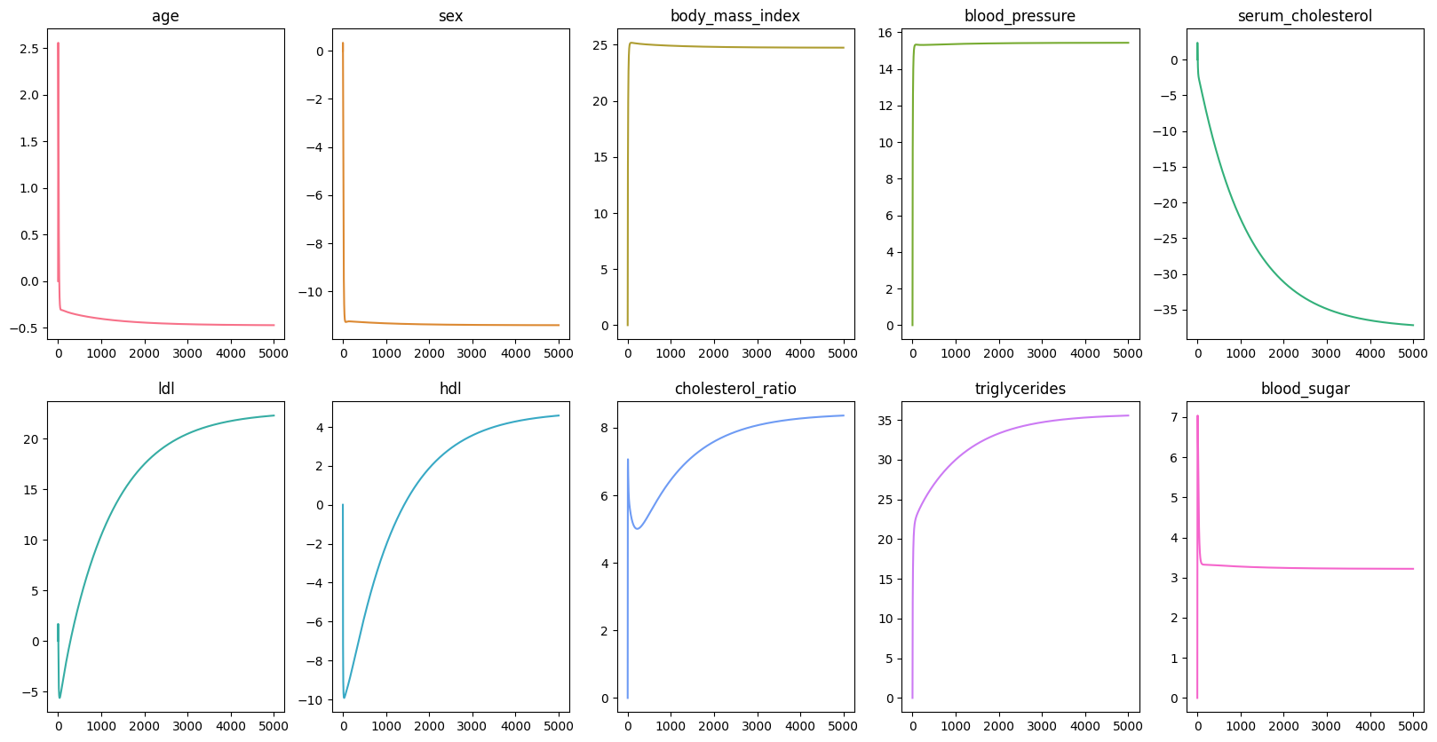
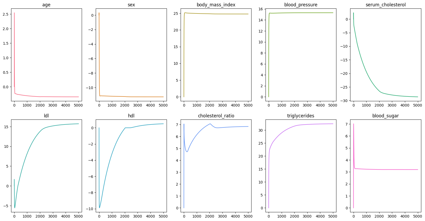
scaler = StandardScaler()X_train_scaled = scaler.fit_transform(X_train)X_test_scaled = scaler.transform(X_test)Now out data is ready, we want pick a number of epoch, meaning how many times our model has to go through the dataset. In this example, we are going to use epochs, and it might take sometime. However, epochs should be enough to see the changes in the loss, intercept, and coefficients. Then we initialize the history of the loss, intercept, and coefficients so that we can visualize the changes in the values of these variables.
epochs = 100_000loss_history = list()intercept_history = list()coefficients_history = np.zeros((scaled_X.shape[1], epochs)) Next, we would need two helper functions: predict and loss_function.
Make sure to use vectorized operations to make the code faster.
Remember, regularization_term is the in the cost function.
Unlike Lasso Regression, the loss function in Ridge Regression is the sum of the squares of the errors plus the sum of the squares of the weights.
def predict(intercept: float, coefficient: list, data: list) -> list: return intercept + np.dot(data, coefficient)
def loss_function(coefficients, errors, regularization_term): return np.mean(np.square(errors)) + regularization_term * np.sum(np.square(coefficients)) We also need a function called soft_threshold to update the coefficients. There are three conditions:
- If the coefficient is less than the negative of the regularization term, then we subtract the regularization term from the coefficient.
- If the coefficient is greater than the regularization term, then we subtract the regularization term from the coefficient.
- If the coefficient is between the negative and positive regularization term, then we set the coefficient to zero.
def soft_threshold(rho, lambda_): if rho < -lambda_: return (rho + lambda_) elif rho > lambda_: return (rho - lambda_) else: return 0def ridge_regression( x, y, epochs, learning_rate = 0.1, regularization_term = 0.001): intercept, coefficients = 0, np.zeros(x.shape[1]) length = x.shape[0]
intercept_history.append(intercept) coefficients_history[:, 0] = coefficients loss_history.append(loss_function(coefficients, y, regularization_term))
for i in range(1, epochs): predictions = predict(intercept, coefficients, x) errors = predictions - y intercept = intercept - learning_rate * np.sum(errors) / length intercept_history.append(intercept)
for j in range(len(coefficients)): gradient = np.dot(x[:, j], errors) / length temp_coef = coefficients[j] - learning_rate * gradient coefficients[j] = soft_threshold(temp_coef, regularization_term) coefficients_history[j, i] = coefficients[j]
loss_history.append( loss_function( coefficients, errors, regularization_term ) )
return intercept, coefficients
intercept, coefficients = ridge_regression(scaled_X, data.target, epochs)Model Comparison
| Baseline | Ours | |
|---|---|---|
| MSE | 2900.07 | 2878.51 |
| age | 1.75 | -0.35 |
| sex | -11.51 | -11.29 |
| body_mass_index | 25.61 | 24.77 |
| blood_pressure | 16.83 | 15.31 |
| serum_cholesterol | -44.32 | -28.79 |
| ldl | 24.54 | 15.84 |
| hdl | 7.62 | 0.56 |
| cholesterol_ratio | 13.12 | 6.86 |
| triglycerides | 35.11 | 32.53 |
| blood_sugar | 2.35 | 3.19 |
By comparing the baseline model and our model, you would be able to see the noticeable differences in the coefficients of the features. However, the Mean Squared Error values differ only by a small amount.


Conclusion
Here are the key takeaways from this post:
- Ridge Regression is a type of linear regression that uses a regularization term to prevent overfitting.
- It uses the sum of the squares of the weights multiplied by the regularization term to minimize coefficients.
- It will set coefficients close to zero but not exactly zero.
- It can be used to select important features in the dataset, just like Lasso Regression.
- It can increase the model’s interpretability, just like Lasso Regression.
For the baseline model, you could see the code here. For own custom Lasso Regression model, you could see the code here.
Reference
- JMP. What is Multicollinearity? https://www.jmp.com/en_is/statistics-knowledge-portal/what-is-multiple-regression/multicollinearity.html
- Scikit-Learn. California Housing Dataset. https://scikit-learn.org/stable/datasets/real_world.html#california-housing-dataset
- StatsModel. Variance Inflation Factor. https://www.statsmodels.org/stable/generated/statsmodels.stats.outliers_influence.variance_inflation_factor.html
- NBSHARE. How to Use Pandas Correlation Matrix. https://www.nbshare.io/notebook/394171759/How-To-Use-Pandas-Correlation-Matrix/