Logistic Regression

What is Logistic Regression?

Logistic Regression is one of many supervised machine learning algorithms, just like Linear Regression. Instead of predicting a continuous value, it predicts the probability of an event happening, or something is true or false. So, this algorithms is mostly used for binary classification problems. Here are the use cases of Logistic Regression:

1. Predict if an email is spam or not.
2. Predict if a credit card transaction is fraudulent or not.
3. Predict if a customer will churn or not.
4. Predict if a patient has cancer or not.

However, it also has the same limitations as Linear Regression, such as:

1. It is a linear model, so it cannot capture complex non-linear relationships. In other words, it assumes that the data is linearly separable.
2. It assumes that the data is independent of each other. In other words, it assumes that the data is not correlated with each other.
3. It is sensitive to outliers.

Mathematics Behind Logistic Regression

First, Logistic Regression still uses Linear Equation used in Linear Regression, and it’s expressed as:

Second, we are going to need Sigmoid function. This funciton’s sole job is to predict by converting the output of the linear equation into a probability value between $0$ and $1$.

where $z = \theta_0 + \theta_1 \times x$. Then the sigmoid function can be rewritten as:

After acquiring the probability value from the Sigmoid function, we can use a threshold value to classify into one or another. To generalize, we can use the following equation to predict the probability of an event occurring:

Once we have the probability of an event occuring, we then use a threshold value to round up the probability value to either $0$ or $1$. If $P(y | x) \geq 0.5$, then the data is classified as $1$, otherwise it is classified as $0$.

Similar to what we did in the Linear Regression post, we need to estimate the best $\theta_0$ and $\theta_1$ using the Gradient Descent algorithm. What the Gradient Descent algorithm does is to update the $\theta_0$ and $\theta_1$ values based on the cost function and the learning rate.

This example is just a simple linear model, we are going to use the following equations to update intercept and coefficient:

where $\alpha$ is the learning rate, $\theta_p$ is the $p$-th parameter, $J$ is the cost function, and $x_p$ is the $p$-th feature.

Since we only have $\theta_0$ and $\theta_1$, we can simplify the equation above to:

Implementation

First things first, we need to import the necessary libraries.

1
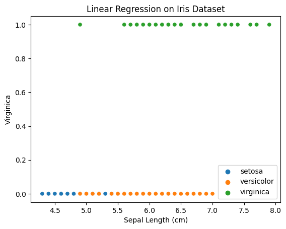
from sklearn.datasets import load_iris
2
import matplotlib.pyplot as plt
3
import seaborn as sns
4
import numpy as np

Say that we only have a feature $x$, the sepal length, and we want to determine the instance is a Virginica or not. Let’s prepare the data.

1
iris = load_iris()
2
sepal_length = iris.data[:, 0]
3
target = iris.target
4

5
is_virginica_dict = {0: 0, 1: 0, 2: 1}
6
is_virginica = np.array([is_virginica_dict[i] for i in target])
7

8
species_dict = {0: 'setosa', 1: 'versicolor', 2: 'virginica'}
9
species_name = np.array([species_dict[i] for i in target])

You might be wondering why we have is_virginica_dict. I need that variable to separate the data so that some data sit at the bottom of the plot and some sit at the top of the plot.

So let’s add a line like we did in the Linear Regression post with $-1.2$ as the intercept and $0.28$ as the coefficient.

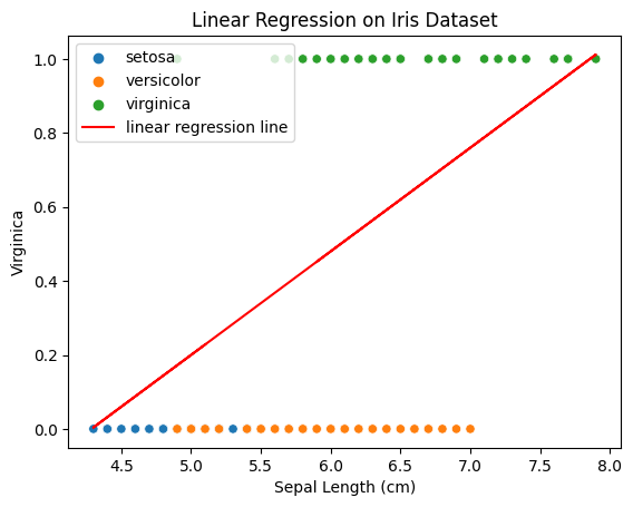
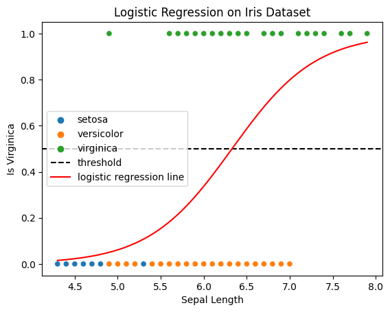
It’s clear that our data do not follow the pattern that the straight line is showing in the graph. Thus, we need to use Sigmoid function to bend the line, so that the line would look like this:

1
def accuracy(y_pred, y):
2
  return np.sum(y_pred == y) / len(y)
3

4
def sigmoid(x):
5
  return 1 / (1 + np.exp(-x))
6

7
def linear_function(intercept, coefficient, x):
8
  return intercept + coefficient * x
9

10
def threshold(x):
11
  return np.where(x > 0.5, 1, 0)
12

13
def gradient_descent(x, y, epochs, alpha = 0.01):
14
  intercept, coefficient = -1.2, 0.28 # initial guess
15

16
  for _ in range(epochs):
17
    y_pred = np.array(
18
      [
19
        sigmoid(
20
          linear_function(intercept, coefficient, i)
21
        ) for i in x
22
      ]
23
    )
24
    intercept = intercept - alpha * np.sum(y_pred - y) / len(y)
25
    coefficient = coefficient - alpha * np.sum((y_pred - y) * x) / len(y)
26

27
  return intercept, coefficient

Let’s train our model for $100,000$ times.

1
intercept, coefficient = gradient_descent(sepal_length, is_virginica, 100000)
2
predicted_value = np.array([sigmoid(linear_function(intercept, coefficient, i)) for i in sepal_length])
3
corrected_prediction = threshold(predicted_value)
4
pred_acc = aaccuracy(corrected_prediction, is_virginica)
5

6
print(f'accuracy: {pred_acc:.4f}') # 0.8
7
print(f'intercept: {intercept:.4f}') # -13.004847396222699
8
print(f'coefficient: {coefficient:.4f}') # 2.0547824850027654

Not bad, the accuracy is $80\%$, with $-13.00$ as the intercept and $2.05$ as the coefficient.

You can find the full code in this repository

Conclusion

1. Logistic Regression is a supervised machine learning algorithm that is used for binary classification problems.
2. It uses the Sigmoid function to calculate the probability of an event occurring.
3. It uses a threshold value to roundup the probability value to either $0$ or $1$. If $\delta(x) > 0.5$, then the data is classified as $1$, otherwise it is classified as $0$.

References

1. Vieira, Tim. Exp-Normalize Trick. https://timvieira.github.io/blog/post/2014/02/11/exp-normalize-trick/
2. IBM. Logistic Regression. https://developer.ibm.com/articles/implementing-logistic-regression-from-scratch-in-python/